RCS and the Race for Quantum Supremacy: A Practical Look at Benchmarks and Real-World Relevance
TL;DR: Google’s Willow chip has smashed
its own Random Circuit Sampling (RCS) benchmarks from the 2019 Sycamore system,
re-igniting talk about quantum supremacy. But do these record-breaking
achievements translate into real-world utility or remain largely symbolic
milestones?
In this post, we’ll dissect Random Circuit Sampling (RCS) as a benchmark and highlight the ways in which claims of quantum supremacy, particularly Google’s recent announcement, can be misleading without demonstrated real-world applicability. While headlines often tout RCS as proof that quantum processors are surpassing classical supercomputers, it’s critical to understand how RCS works and why it may not directly reflect practical applications. We’ll walk through how RCS experiments are set up, why they’re considered so hard for classical machines, and where these benchmarks do and don’t align with real-world applications. Along the way, we’ll highlight the nature of quantum vs. classical “randomness,” and discuss what these milestones truly mean for the future of quantum computing. By the end, you’ll not only see how RCS generates millions of “bitstrings” in minutes but also appreciate why researchers are still wrestling with the question: is quantum supremacy just around the corner, or do we need more practical tasks to see genuine quantum advantage?
Introduction
Recently, Google announced that its new “Willow” quantum chip surpassed the record-breaking Random Circuit Sampling (RCS) metrics once achieved by the 2019 “Sycamore” system - further amplifying the buzz around quantum supremacy. RCS, in essence, involves running complex, randomly generated quantum circuits on a real device to see if it can produce results faster or more accurately than a classical computer can simulate. The fanfare surrounding these new benchmarks, however, raises an important question: how meaningful is RCS for gauging quantum computing’s readiness for real-world applications?
What is RCS?
Random Circuit Sampling (RCS) involves sampling from the output distribution of a randomly generated quantum circuit, i.e. a random placement of quantum gates, and comparing the empirical distribution to what classical simulation would predict. When the circuit depth and qubit count exceed the classical computability threshold, it can serve as an empirical demonstration of quantum supremacy.
The Issues with the RCS Benchmark
Despite the hype, there’s a lot that can be criticised about the whole RCS benchmark being used to demonstrate quantum supremacy:
- Non-verifiability for large circuits
- Problem: For big RCS experiments (like Willow), classical simulation times can balloon to astronomical estimates (10^25 years or more).
- Impact: Direct, exact verification of the quantum output is impossible in practice (as it would take 10^25 years), so researchers rely on partial checks (smaller circuits, approximate simulations) and statistical extrapolation, which introduces uncertainty.
- Limited practical utility
- Problem: RCS is purpose-built to stump classical computers rather than solve real problems (like optimization or simulating molecules).
- Impact: While it proves certain quantum devices can handle large random circuits, industry and science gain little direct benefit - no immediate breakthroughs in anything of scientific benefit.
- Intentionally “unfair” setup
- Problem: RCS is constructed to exploit quantum parallelism while presenting an exponential challenge to classical simulation.
- Impact: It shows a “win” for quantum hardware on a contrived task, raising questions about “supremacy” claims for more general or commercial applications.
- Sensitivity to hardware noise
- Problem: Real quantum devices have error rates (gate errors, readout noise) that degrade fidelity.
- Impact: Achieving a distribution close to the ideal quantum output can be extremely challenging, especially at larger circuit depths. If noise dominates, it undercuts the very point of the benchmark.
- Near-impossibility of targeted error correction
- Problem: For highly structured quantum algorithms, engineers can weave error-correction routines or targeted mitigation strategies into the known gate sequence. But with random circuits, there’s no predictable structure or “map” that specifies which qubits will interact when and how - the gates are randomly placed after all and don’t perform any algorithm at all.
- Impact: Effective error correction usually relies on periodic syndrome measurements and well-defined layouts. In a random layout, errors can accumulate rapidly across qubits in ways that are far harder to track or correct. As a result, small imperfections can derail the output distribution much more significantly in RCS than they might in a more controlled algorithmic sequence. Add this to the non-verifiability mentioned as our first issue and you can see the claims of correctness from Willow’s processing can become doubtful.
- Difficult interpretation of “Quantum Supremacy”
- Problem: RCS experiments can yield exciting headlines (“Quantum beats classical!”), yet the phrase “quantum supremacy” is often misunderstood.
- Impact: This can oversell the state of quantum tech to the public and policymakers, conflating a single contrived task with general-purpose capabilities or “quantum advantage.”
- Media hype and miscommunication
- Problem: RCS often appears in the press as “Quantum Computer Slays Supercomputer at Complex Task,” overshadowing nuances.
- Impact: This creates unrealistic expectations, potentially alienating researchers or industries looking for near-term, real-world ROI. The discussion of this alone could fill an entire post - just try a media search and you will see how much repetitious hyperbole was used around the time of the announcement. Then there’s irrational exuberance applied to any and all stocks related to quantum computing. What’s to say that these won’t come crashing down from their infinite P/E ratios in a few months’ time?
In short, while RCS is an important stress test and a marquee demonstration for quantum hardware capability, it comes with intrinsic caveats around verification, real-world utility, and fairness that limit its broader significance.
However, let’s remain positive and not overly critical; let’s move onto looking at how the experiment is constructed so that we can seek to reproduce it albeit at a much smaller scale…
Experimental Process Flow
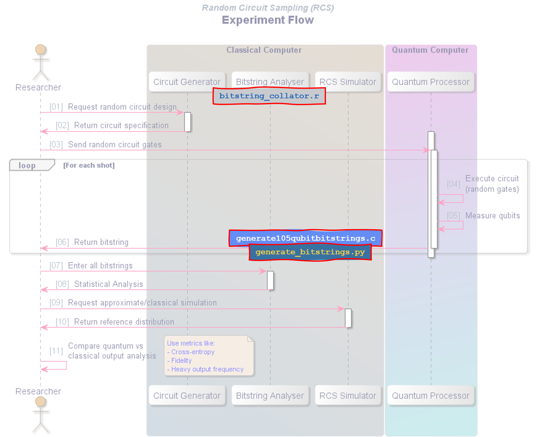
Below is a simplified sequence flow diagram illustrating an RCS experiment. In an actual research or industrial setting, each of these steps could involve far more complexity - multiple layers of error correction, control systems, and in-depth post-processing. However, for educational purposes, this high-level view helps clarify the core responsibilities: how a random circuit is generated and sent to the quantum computer, how the qubits are measured repeatedly (each measurement yielding a bitstring), and how classical analysis then compares the quantum outputs against a reference distribution. This streamlined sequence is a handy reference for understanding the basic workflow behind RCS, without the overhead of real-world engineering details.

The process begins when the Researcher requests a random circuit design from the Circuit Generator running on a conventional (classical) computer. Once that specification is returned, the Researcher sends these circuit instructions to the Quantum Processor. The Quantum Processor then executes the specified random gates on its qubits for each shot, measures the resulting bitstring, and returns these bitstrings back to the Researcher. This loop of “execute → measure → return bitstring” continues until sufficient shots have been run to build up a meaningful output distribution.
Back on the classical side, the Researcher sends these bitstrings to the Bitstring Analyser, which performs statistical checks - counting how often each bitstring appears and detecting patterns or “heavy outputs”. In parallel, the Researcher asks the RCS Simulator for a reference distribution, but since a full classical simulation is typically feasible only for small circuits, it may be an approximation.
Finally, the Researcher compares the measured quantum distribution against the classical reference, using metrics like cross-entropy, fidelity, or heavy-output frequency. This comparison step helps validate whether the quantum device’s results align with the idealized model of the circuit, providing insight into both the quantum hardware’s performance and the challenge of simulating it on classical machines.
Our Toy RCS Experiment: From Random Bitstrings to Mock Distribution Analysis
Below you’ll see our RCS process flow diagram again, but this time with our custom scripts overlaid on the relevant steps. This illustrates how we move from Python scripts that generate simplistic random bitstrings, through the C program (generate105qubitbitstrings.c) which creates a more “quantum-like” output at Step 6, to the R script that collates all returned bitstrings and builds a histogram of their frequencies. By matching each program to the appropriate stage in the sequence (e.g., circuit generation, repeated measurement, and final statistical analysis), we replicate key elements of an RCS experiment - even if our toy examples can’t come anywhere close to the complexity of real quantum hardware or the reference classical simulator.
Purely Random Bitstring Generation
This Python script below is about as straightforward as it gets: it takes two arguments - “num_qubits” (the length of each bitstring) and “num_shots” (the total number of bitstrings to generate). Then it simply loops “num_shots” times, each time printing out a randomly generated string of 0s and 1s. Although it’s dubbed “naive,” it’s a perfect baseline demonstration for how raw bitstring sampling might look in an RCS-style experiment - except it’s purely uniform random and has no correlation between qubits or shots. Running it with large arguments can produce massive files, as we’ll see below.
def main():
parser = argparse.ArgumentParser(
description="Generate random bitstrings given number of qubits and
shots."
)
parser.add_argument("num_qubits", type=int, help="Number of qubits (bitstring
length)")
parser.add_argument("num_shots", type=int, help="Number of
bitstrings to generate")
args
= parser.parse_args()
num_qubits = args.num_qubits
num_shots = args.num_shots
for _ in range(num_shots):
# Generate a random bitstring of length 'num_qubits'
bits = ''.join(str(random.randint(0, 1)) for _ in range(num_qubits))
print(bits)
Here, we ran the script with 105 qubits and 18.9 million
shots to replicate the data output of Google’s Willow experiment, in size at
least. The command took just over 34 minutes of real time, though the “user”
and “sys” times are minimal because the process is mostly waiting on I/O.
Willow produced this quantity of data in under 5 minutes.
07:39:40 User@AN20 ~/QuantumBenchmark
980 0 😊 $
time ./generate_bitstrings.py 105 18900000 >
105qubit_bitstrings.txt
real
34m41.455s
user
0m0.046s
sys
0m0.061s
Finally, to confirm, we see that “wc -l” reports exactly 18,900,000 lines in the output, each line being a 105-bit string, yielding a total file size of roughly 1.9 GB. This not only indicates we successfully generated the intended number of bitstrings, but also highlights how quickly these experiments can produce huge datasets. In a real RCS experiment, the quantum machine’s measurement shots can likewise accumulate staggering amounts of output data, though the distribution (and hence the challenge in reproducing it classically) is often far more complex.
08:16:58 User@AN20 ~/QuantumBenchmark
218 0 😊 $
wc -l 105qubit_bitstrings.txt
18900000 105qubit_bitstrings.txt
08:36:59 User@AN20 ~/QuantumBenchmark
419 0 😊 $
du -h 105qubit_bitstrings.txt
1.9G
105qubit_bitstrings.txt
Bitstring Analysis
The following R script (bitstring_collator.r) demonstrates a simple approach to reading a large text file of bitstrings, computing the frequency of each unique string, and visualizing the results. It’s designed to handle millions of lines, though as we’ll see, memory usage can grow quickly if each bitstring is unique (as in a purely random dataset). The script also produces basic statistics - like how many total shots were recorded, how many distinct bitstrings were found, and the top five most frequent bitstrings - before plotting a histogram (in probability form).
# Parse
Command-Line Argument(s)
args <- commandArgs(trailingOnly = TRUE)
if (length(args) < 1) {
stop("Usage: Rscript
bitstring_collator.R <bitstrings.txt
file>")
}
bitstring_file <- args[1]
# Read
Bitstring Data
bitstrings <- readLines(bitstring_file)
cat(
"Size
of 'bitstrings' object:",
format(object.size(bitstrings), units = "auto"), "\n"
)
# Calculate
Frequencies
freq_table <- table(bitstrings) # table() gives you counts of each
unique bitstring
df_freq <- as.data.frame(freq_table) # convert table to data frame
colnames(df_freq) <- c("bitstring", "count")
# Compute
Probabilities
df_freq$prob <- df_freq$count / sum(df_freq$count)
# Print
Basic Stats
cat("Total Shots:", sum(df_freq$count), "\n")
cat("Unique
Bitstrings:", nrow(df_freq), "\n\n")
# Show the
top 5 most common bitstrings
df_freq_sorted <- df_freq[order(-df_freq$count),]
cat("Top 5 Most
Frequent Bitstrings:\n")
print(head(df_freq_sorted, 5))
# Plot
Histogram of counts or probabilities
suppressPackageStartupMessages(library(ggplot2))
p <- ggplot(df_freq, aes(x = bitstring, y = prob)) +
geom_bar(stat = "identity", fill = "steelblue") +
labs(
title = "Histogram of Measured Bitstrings",
x = "Bitstring",
y = "Probability"
) +
theme_minimal()
# Save the
Plot
output_file <- gsub("\\.bits$", ".histogram.png", bitstring_file)
cat("Saving histogram
to", output_file, "\n\n")
ggsave(output_file, p, width = 16, height = 9)
By running bitstring_collator.r on our massive 18.9 million line file of 105-qubit bitstrings, we quickly see the practical impacts of storing so many unique strings in memory. The script reports 3.2 GB of memory usage just to load the dataset - reflecting the fact that each 105-bit string is stored as a long character vector in R. We also observe that every shot is unique (18.9 million unique strings), confirming that the purely random generator had zero collisions. The script was interrupted before it attempted to draw the histogram - it would have “flat-lined” at y=1 for 18.9 million values of x.
08:17:08 User@AN20 ~/QuantumBenchmark
228 0 😊 $
time ./bitstring_collator.R
105qubit_bitstrings.txt
Size of 'bitstrings' object: 3.2 Gb
Total Shots: 18900000
Unique Bitstrings: 18900000
real
18m50.782s
user
0m0.000s
sys
0m0.046s
The Vastness of the State Space
To get a sense of scale, 2105 is approximately 4.03×1031 - that’s a 4 followed by 31 zeros. Put another way, there are more possible states in 105 qubits than there are stars in the observable universe by many orders of magnitude. This is why even 18.9 million samples barely scratches the surface of such an enormous space, and why collisions are so unlikely when the distribution is nearly uniform.
And to get a rough sense of how many times we would have to produce 18.9 million 105-bit strings before expecting even one collision, we can invoke the birthday paradox. In a uniform distribution of size 2105, the expected number of draws needed for a ~50% chance of collision is on the order of:
$$ \sqrt{2^{105}} = 2^{\frac{105}{2}} \approx 2^{52.5} \approx 6.4 \times 10^{15} $$
Each block of 18.9 million (1.89×10⁷) bitstrings is one “batch” of draws. So, the number of batches needed for an expected collision is roughly:
$$ \frac{6.4 \times 10^{15}}{1.89 \times 10^7} \approx 3.4 \times 10^8 \approx 340 \text{ million} $$
Putting That in Perspective
- Total bitstrings:
$$ 3.4 \times 10^8 \times 1.89 \times 10^7 \approx 6.4 \times 10^{15} $$
- Total data size (if each batch is ~1.9 GB):
$$ 3.4 \times 10^8 \times 1.9GB \approx 6.5 \times 10^8 GB \approx 650PB $$
- That’s several hundred thousand consumer hard disks: enough
to store all of Netflix’s content (approx. 20,000 titles) nearly 8,000
times; Spotify’s library of 100 million songs, 6,000 times; 1,500 copies
of the full Wikipedia; 60,000 copies of Steam’s game catalogue; and almost
all of Instagram or Facebook[1].
As for scientific data, 11,000 years of Hubble data, 31,00 years of JWST
and about 20 years of CERN’s output
- Total time: If each batch took ~30–35 minutes in our Python
script, it’d take about 20,000 years to produce a batch of 105-qubit
bitstrings (with each batch being 18.9 million) to expect to get just one
collision.
This is why, in purely uniform sampling
of 105-bit outputs, collisions are basically never observed for any realistic
number of shots. In the next example, when we introduce skew or “heavy”
outputs, we’ll see how this same R script can reveal drastically different
patterns of repetition and collisions.
Beyond Uniform Randomness: A Toy RCS Generator in C
After experimenting with our naive Python
bitstring generator, we learned two important lessons:
- Pure uniform randomness across 105-bit strings leads to
virtually no collisions in tens of millions of samples, making it a poor
analogue for real RCS outcomes.
- Handling data at scale - both in memory and I/O - can
become a major bottleneck if every bit is naively stored as an entire
character.
To address these points, we turn to a
C-based approach. First, we introduce non-uniform distributions (log-normal
amplitudes) to ensure some “heavy” bitstrings appear more often. Second, we
store each 105-bit pattern in 14 bytes rather than the earlier 105 bytes,
packing bits and avoiding the inefficiency of strings. The resulting program
still can’t replicate the full complexity of a quantum circuit’s output, but it
produces a more skewed distribution - helping us see collisions, large-scale
repetition, and other phenomena reminiscent of real RCS experiments.
Here are some key snippets from the
program:
Th Box–Muller
transform function draws two uniform [0,1] samples
(u1, u2) and converts them to a Gaussian
(μ=0, σ=1) random number. The program uses this to create a log-normal
amplitude later, which helps shape the distribution of output strings so some
appear more frequently - mimicking a skewed, RCS-like distribution.
static double rand_normal()
{
double u1 = (double)rand() / (double)RAND_MAX;
double u2 = (double)rand() / (double)RAND_MAX;
double r = sqrt(-2.0 * log(u1));
double theta = 2.0 * M_PI * u2;
double z = r * cos(theta); // normal(0,1)
return z;
}
The following code assigns a log-normal amplitude to each pattern. The squaring that amplitude makes the distribution even more skewed, so a small fraction of patterns end up with disproportionately high probability. It then cumulatively sums these weights and normalizes them, building a Cumulative Distribution Function (CDF).
for (int i = 0; i < subset_size; i++)
{
double z = rand_normal(); // normal(0,1)
double amplitude = exp(z); // log-normal(0,1), a positive value
double w = amplitude * amplitude; // square for a more pronounced weight
weights[i] = w;
}
…
for (int i = 0; i < subset_size; i++)
{
running += weights[i];
cdf[i] = running / sum_w; // normalized
}
By sampling from this CDF, the program
enforces that high-weight patterns appear more often in the final output file -
similar to how some bitstrings in an RCS experiment
can have a higher amplitude (and thus higher probability).
Each shot picks a random double r ∈
[0,1] and searches the CDF to find which pattern’s probability
range it falls into. This binary search makes lookups O(log
n) rather than O(n) - important if subset_size is
large.
static int find_index_in_cdf(const double *cdf, int size, double r)
{
int left = 0;
int right = size - 1;
while (left < right)
{
int mid = (left + right) / 2;
if (cdf[mid] < r)
{
left = mid + 1;
}
else
{
right = mid;
}
}
return left; // left == right => the position
}
Together, these snippets show how the C program creates a nonuniform, skewed distribution of 105-bit strings. It’s just a toy version of “random circuit sampling” - instead of deriving probabilities from an actual quantum circuit, it uses log-normal weights to produce “heavy outputs.” The goal is to generate collisions and an uneven histogram that’s a bit more representative of realistic (but still vastly simplified) quantum RCS outputs.
Here is the compiled C program being run with
a subset size of 10,000 and our usual 18.9 million shots (in keeping with the
Willow experiment) followed by the bitstring_collator.r script:
06:28:21 User@AN20 ~/QuantumBenchmark
101 0 😊 $
time ./generate105qubitbitstrings.exe 10000 18900000
105qubit_lognormal_bitstrings.txt
real
3m10.805s
user
3m6.796s
sys
0m0.859s
07:37:30 User@AN20 ~/QuantumBenchmark
250 0 😊 $
time ./bitstring_collator.R
105qubit_lognormal_bitstrings.txt
Size of 'bitstrings' object: 145.9 Mb
Total Shots: 18900000
Unique Bitstrings: 9955
Top 5 Most Frequent Bitstrings:
bitstring
7865
110010000000111001001001000110110101011110000101000111110100101000100011111001011001010000001010100011000
5343
100001110010000101101010010001011011100001010001110100010010110011001111010111101101000010101000110011000
1854
001011110000001100101000110111000010000001000011001110110010110100101111010010010111110001100000101110011
3337
010101000101001101111111010101001000000011011111011110100110101110100110111001111111110010100001001100001
503
000011001101001110001111011101101001101001001110011110010001000001100101111010101101100010001000101001111
count prob
7865 737499 0.039021111
5343 371077 0.019633704
1854 280379 0.014834868
3337 204757 0.010833704
503 170701 0.009031799
real
0m25.798s
user
0m0.000s
sys
0m0.015s
Notice several important differences
compared to the Python scenario:
- Faster Generation
- The C program finishes in just 3 minutes and 10 seconds
for 18.9 million shots, showcasing the efficiency of bit-packing, streamlined
data structures and the pure speed of C.
- Memory and Collisions
- The R script reports ~146 MB to store all 18.9 million
lines, which is far less than the 3.2 GB from the uniform dataset. This
is largely because we now have only 9,955 unique bitstrings (versus 18.9
million previously). The top 5 alone accumulate substantial counts,
demonstrating a non-uniform, highly skewed distribution.
- Representative “Heavy Outputs”
- Some bitstrings appear hundreds of thousands of times,
each with a probability of a few percent. This stands in sharp contrast
to the 1-to-1 mapping of uniform generation, where collisions were non-existent.
Overall, this more realistic (though
still toy) approach illustrates how skew in the distribution can force actual
repetition and a “heavy-tail” effect - vaguely mirroring the kind of output
that might arise from an actual Random Circuit Sampling experiment on quantum
hardware.
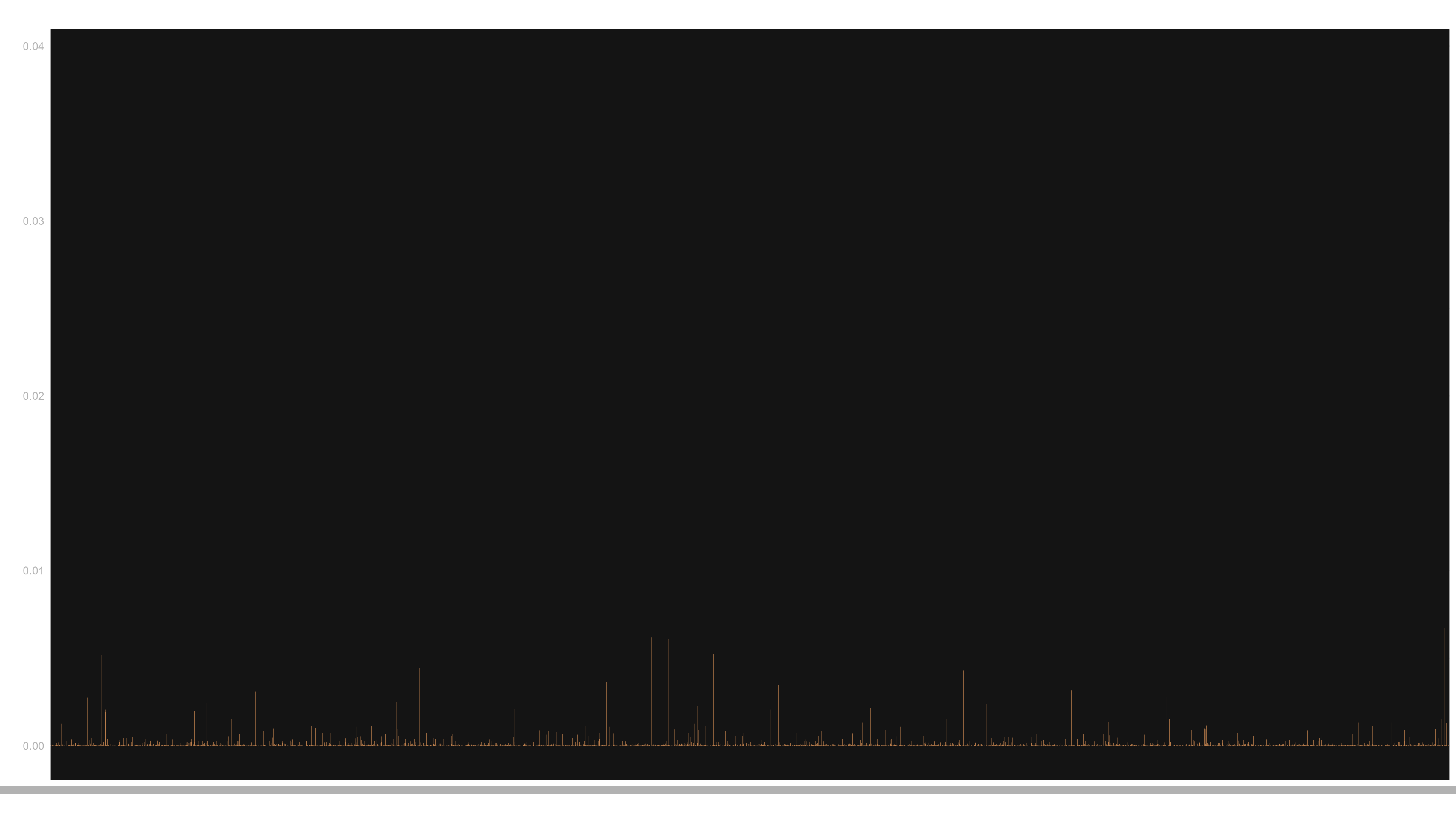
Finally, here is the histogram generated
by the R script:
Conclusion
In this article, we replicated the basic
flow of a Random Circuit Sampling experiment- albeit in a toy fashion. We
showed how uniform random bitstrings fail to capture any real collisions and
how a lognormal-based approach in C yields a more skewed distribution that
hints at the kind of “heavy outputs” often reported in true RCS studies. By
using Python for naive generation, a C program for more nuanced sampling, and R
for collation and histogram analysis, we illustrated several key lessons:
- Scale Matters: Even tens of millions of bitstrings barely
graze the surface of a 105-bit space, making collisions extraordinarily
rare without a skewed distribution.
- Data Handling: Bit-packing and more efficient I/O can
drastically reduce run times and memory usage compared to naive
approaches.
- Skew Produces Meaningful Repetitions: A non-uniform
distribution - though still contrived - reveals the collisions and “heavy
outputs” more akin to quantum sampling than a purely flat distribution.
The [F]utility of RCS Benchmarking
Yet, it’s important to recognize the limitations of RCS itself. The benchmark is intentionally designed to be hard for classical computers but more “natural” for quantum devices. In this sense, it serves as a theoretical stress test rather than a practical solution to a real-world computational need. Some argue that this mismatch renders RCS an unfair comparison: it doesn’t address industrial problems like optimization or cryptography, yet it trumpets “supremacy” simply because classical simulation at large scale becomes infeasible.
At the same time, RCS has value as a demonstration of hardware maturity - showing that qubits can generate massive, complex distributions no known classical machine can match. But its “[f]utility” lies in the fact that, while it makes for a bold headline, it doesn’t immediately translate into breakthroughs in commercial or scientific fields. Instead, RCS is a niche benchmark that leverages quantum effects in a contrived setting, making it a spectacular but ultimately futile show of power.
What’s Next
Looking ahead, we’ll push beyond purely
synthetic datasets. In our next post, we’ll generate actual random quantum
circuits, run them on a small, real quantum processor, and compare those
outputs against a well-established classical simulator. Naturally, we’re
limited to only a few qubits, as large-scale classical simulation remains out
of reach for everyone - even Google. Still, it’s a vital step toward
understanding the true nature of quantum supremacy claims: not only how quantum
devices handle contrived tasks, but also whether these insights hint at future,
genuinely useful quantum applications.